7 Data warehouse contains historical data and is used to analyze business performance
As our bike part seller business grows (that we saw in the setup chapter), we will want to analyze data for various business goals.
Sellers will also want to analyze performance and trends to optimize their inventory. Some of these questions may be
- Who are the top 10 sellers, who have sold the most items?
- What is the average time for an order to be fulfilled?
- Cluster the customers who purchased the same/similar items together.
- Create a seller dashboard that shows the top-performing items per seller
These questions ask about things that happened in the past, require reading a large amount of data, and aggregating data to get a result. Most companies generate large amounts of data and need to analyze it effectively. Starting out by using your company’s backend database is a viable approach. As the size of data and complexity of your systems and queries increase, you will want to use databases specifically designed for large-scale data analytics, known as OLAP systems.
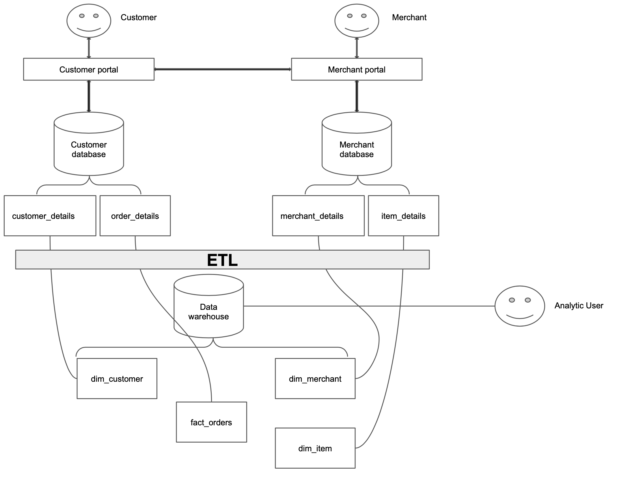
A data warehouse is a database that stores all your company’s historical data.
While your upstream systems can be a single service, or multiple microservices and typically does not store historical change, a warehouse is designed to be the single source of truth of all the historical information you’d need about your company. See the simple example below:
7.1 OLTP vs OLAP-based data warehouses
There are two primary types of databases: OLTP (Online Transaction Processing) and OLAP (Online Analytical Processing). Their differences are shown below.
| OLTP | OLAP | |
|---|---|---|
| Stands for | Online transaction processing | Online analytical processing |
| Usage pattern | Optimized for fast CRUD(create, read, update, delete) of a small number of rows | Optimized for running select c1, c2, sum(c3),.. where .. group by on a large number of rows (aka analytical queries), and ingesting large amounts of data via bulk import or event stream |
| Storage type | Row oriented | Column-oriented |
| Data modeling | Data modeling is based on normalization | Data modeling is based on denormalization. Some popular ones are dimensional modeling and data vaults |
| Data state | Represents current state of the data | Contains historical events that have already happened |
| Data size | Gigabytes to Terabytes | Terabytes and above |
| Example database | MySQL, Postgres, etc | Clickhouse, AWS Redshift, Snowflake, GCP BigQuery, etc |
Note Apache Spark started as a pure data processing system, and over time, with the increased need for structure, it introduced capabilities to manage tables.
7.2 Column encoding enables efficient processing of a small number of columns from a wide table
The significant improvement in analytical queries on OLAP is attributed to its column-store technique. Let’s consider a table items, with the data shown below.
| item_id | item_name | item_type | item_price | datetime_created | datetime_updated |
|---|---|---|---|---|---|
| 1 | item_1 | gaming | 10 | ‘2021-10-02 00:00:00’ | ‘2021-11-02 13:00:00’ |
| 2 | item_2 | gaming | 20 | ‘2021-10-02 01:00:00’ | ‘2021-11-02 14:00:00’ |
| 3 | item_3 | biking | 30 | ‘2021-10-02 02:00:00’ | ‘2021-11-02 15:00:00’ |
| 4 | item_4 | surfing | 40 | ‘2021-10-02 03:00:00’ | ‘2021-11-02 16:00:00’ |
| 5 | item_5 | biking | 50 | ‘2021-10-02 04:00:00’ | ‘2021-11-02 17:00:00’ |
Let’s see how this table will be stored in a row- and column-oriented storage system. Data is stored as continuous pages (a group of records) on the disk.
Row-oriented storage:
Let’s assume that there is one row per page.
Page 1: [1,item_1,gaming,10,'2021-10-02 00:00:00','2021-11-02 13:00:00'],
Page 2: [2,item_2,gaming,20,'2021-10-02 01:00:00','2021-11-02 14:00:00']
Page 3: [3,item_3,biking,30, '2021-10-02 02:00:00','2021-11-02 15:00:00'],
Page 4: [4,item_4,surfing,40, '2021-10-02 03:00:00','2021-11-02 16:00:00'],
Page 5: [5,item_5,biking,50, '2021-10-02 04:00:00','2021-11-02 17:00:00']
Column-oriented storage:
Let’s assume that there is one column per page.
Page 1: [1,2,3,4,5],
Page 2: [item_1,item_2,item_3,item_4,item_5],
Page 3: [gaming,gaming,biking,surfing,biking],
Page 4: [10,20,30,40,50],
Page 5: ['2021-10-02 00:00:00','2021-10-02 01:00:00','2021-10-02 02:00:00','2021-10-02 03:00:00','2021-10-02 04:00:00'],
Page 6: ['2021-11-02 13:00:00','2021-11-02 14:00:00','2021-11-02 15:00:00','2021-11-02 16:00:00','2021-11-02 17:00:00']
Let’s see how a simple analytical query will be executed.
SELECT item_type,
    SUM(price) total_price
FROM items
GROUP BY item_type;
In a row-oriented database
- All the pages will need to be loaded into memory
- Sum
pricecolumn for the sameitem_typevalues
In a column-oriented database
- Only pages 3 and 4 will need to be loaded into memory. The information on pages 3 and 4, including item_type and total_price, will be encoded in the column-oriented file and also stored in an OLTP called metadata db.
- Sum
pricecolumn for the sameitem_typevalues
As you can see from this approach, we only need to read 2 pages in a column-oriented database, compared to 5 pages in a row-oriented database. In addition to this, a column-oriented database also provides
- Better compression, as similar data types follow each other and can be compressed more efficiently.
- Vectorized processing
All of these features make a column-oriented database an excellent choice for storing and analyzing large amounts of data.