3 Use window function when you need to use values from other rows to compute a value for the current row

Window functions allow you to operate on a set of rows at a time and produce output that has the exact grain as the input (vs GROUP BY, which operates on a set of rows, but also changes the meaning of an output row).

Let’s explore why we might need window functions instead of a GROUP BY.

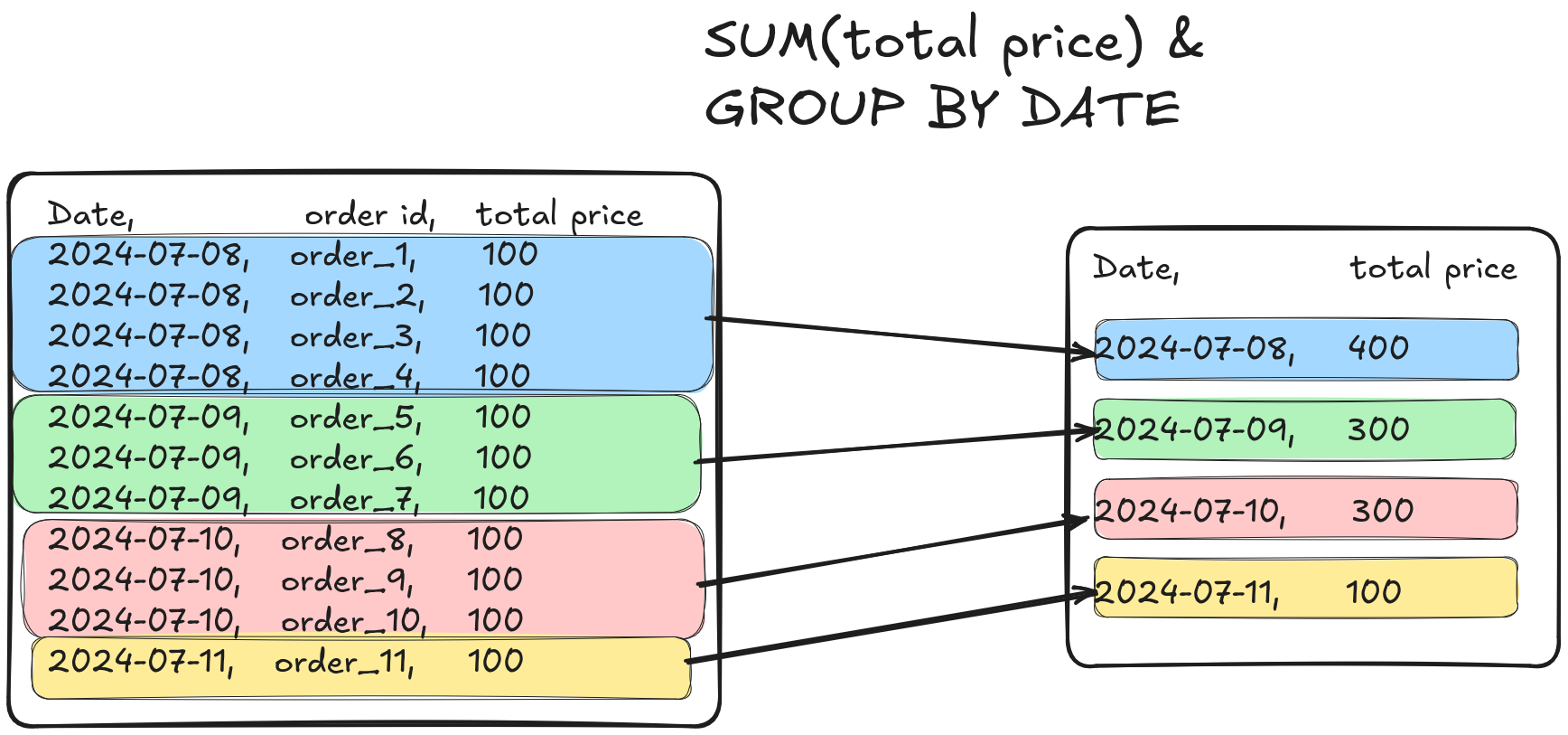
NOTE Notice how GROUP BY changes granularity, i.e., the input data had one row per order (aka order grain or order level), but the output had one row per date (aka date grain or date level).

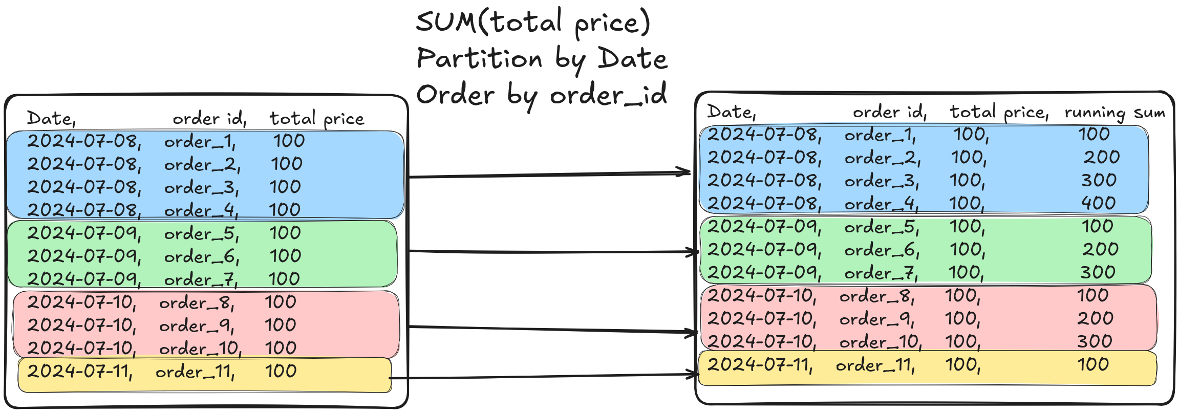
When you perform some operation that requires data from multiple rows to produce the data for one row, without changing the grain, Window functions are almost always a good fit.

Common scenarios when you want to use window functions:

Calculate running metrics/sliding window over rows in the table (aggregate functions)
Ranking rows based on values in column(s) (ranking functions)
Access other rows’ values while operating on the current row (value functions)
Any combination of the above

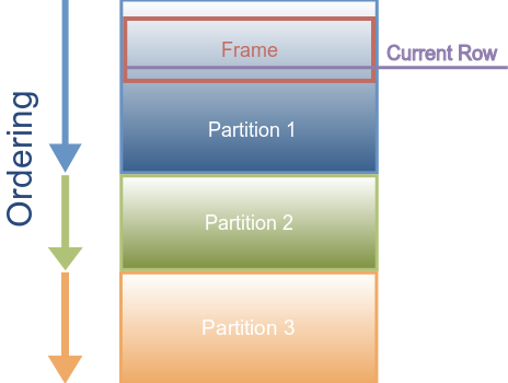
3.1 Window functions have four parts

Partition: Defines a set of rows based on specified column(s) value. If no partition is specified, the entire table is considered a partition.
Order By: This optional clause specifies how to order the rows within a partition. This is an optional clause; without this, the rows inside a partition will not be ordered.
Function: The function to be applied to the current row.
Window frame: Within a partition, a window frame allows you to specify the rows to be considered in the function computation. This enables more options for choosing which rows to apply the function to.

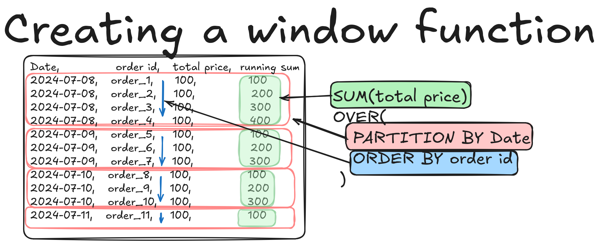
%%sql
use prod.db

%%sql
SELECT
  o_custkey,
  o_orderdate,
  o_totalprice,
  SUM(o_totalprice) -- FUNCTION 
  OVER (
    PARTITION BY
      o_custkey -- PARTITION
    ORDER BY
      o_orderdate -- ORDER BY; ASCENDING ORDER unless specified as DESC
  ) AS running_sum
FROM
  orders
WHERE
  o_custkey = 4
ORDER BY
  o_orderdate
LIMIT
  10;

The function SUM used in the above query is an aggregate function. Notice how the running_sum adds up (i.e., aggregates) the o_totalprice across all rows. The rows themselves are ordered in ascending order by their orderdate.

Reference: The standard aggregate functions are MIN, MAX, AVG, SUM, & COUNT, modern data systems offer a variety of powerful aggregation functions. Check your database documentation for available aggregate functions. e.g., list of agg functions available in TrinoDB

Let’s look at an example: Write a query to calculate the daily running average of the total price for every customer.

Hint: Figure out the PARTITION BY column first, then the ORDER BY column, and finally the FUNCTION to use to compute the running average.

%%sql
SELECT
  o_custkey,
  o_orderdate,
  o_totalprice,
  AVG(o_totalprice) -- FUNCTION 
  OVER (
    PARTITION BY
      o_custkey -- PARTITION
    ORDER BY
      o_orderdate -- ORDER BY; ASCENDING ORDER unless specified as DESC
  ) AS running_sum
FROM
  orders
WHERE
  o_custkey = 4
ORDER BY
  o_orderdate
LIMIT
  10;

3.2 Use window frames to define a set of rows to operate on

While our functions operate on the rows in the partition a window frame provides more granular ways to operate on a select set of rows within a partition.

When we need to operate one a set of rows within a parition (e.g. a sliding window) we can use the window frame to define these set of rows.

Let’s look at an example: Consider a scenario where you have sales data, and you want to calculate a 3-day moving average of sales within each store:

%%sql
SELECT
    store_id,
    sale_date,
    sales_amount,
    AVG(sales_amount) OVER (
        PARTITION BY store_id
        ORDER BY sale_date
        ROWS BETWEEN 2 PRECEDING AND CURRENT ROW
    ) AS moving_avg_sales
FROM
    sales;

In this example:

PARTITION BY store_id ensures the calculation is done separately for each store.
ORDER BY sale_date defines the order of rows within each partition.
ROWS BETWEEN 2 PRECEDING AND CURRENT ROW specifies the window frame, considering the current row and the two preceding rows to calculate the moving average.

Without defining the window frame, the function will consider all rows in the partition up to the current row to compute the moving_avg_sales.

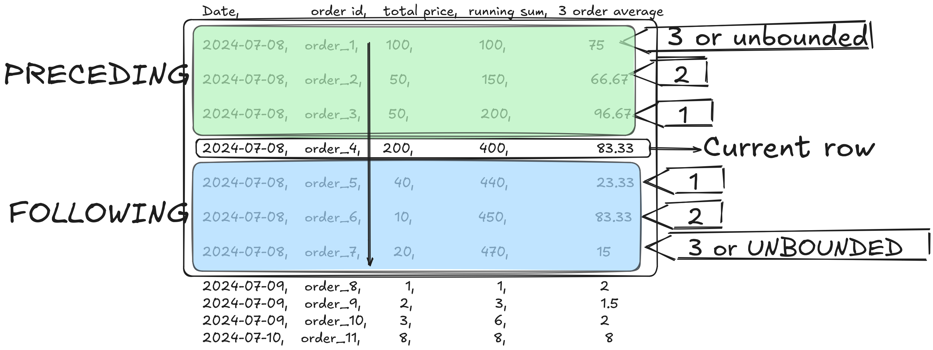
3.2.0.1 Use the ordering of rows to define your window frame with the ROWS clause

ROWS: Used to select a set of rows relative to the current row based on position.
1. Row definition format: ROWS BETWEEN start_point AND end_point.
2. The start_point and end_point can be any of the following three (in the proper order:
  1. n PRECEDING: n rows preceding the current row. UNBOUNDED PRECEDING indicates all rows before the current row.
  2. n FOLLOWING: n rows following the current row. UNBOUNDED FOLLOWING indicates all rows after the current row.

Let’s see how relative row numbers can be used to define a window range.

Consider this window function.

AVG(total_price) OVER ( -- FUNCTION: RUNNING AVERAGE
    PARTITION BY o_custkey -- PARTITIONED BY customer
    ORDER BY order_month 
    ROWS BETWEEN 1 PRECEDING AND 1 FOLLOWING -- WINDOW FRAME DEFINED AS 1 ROW PRECEDING TO 1 ROW FOLLOWING
    )

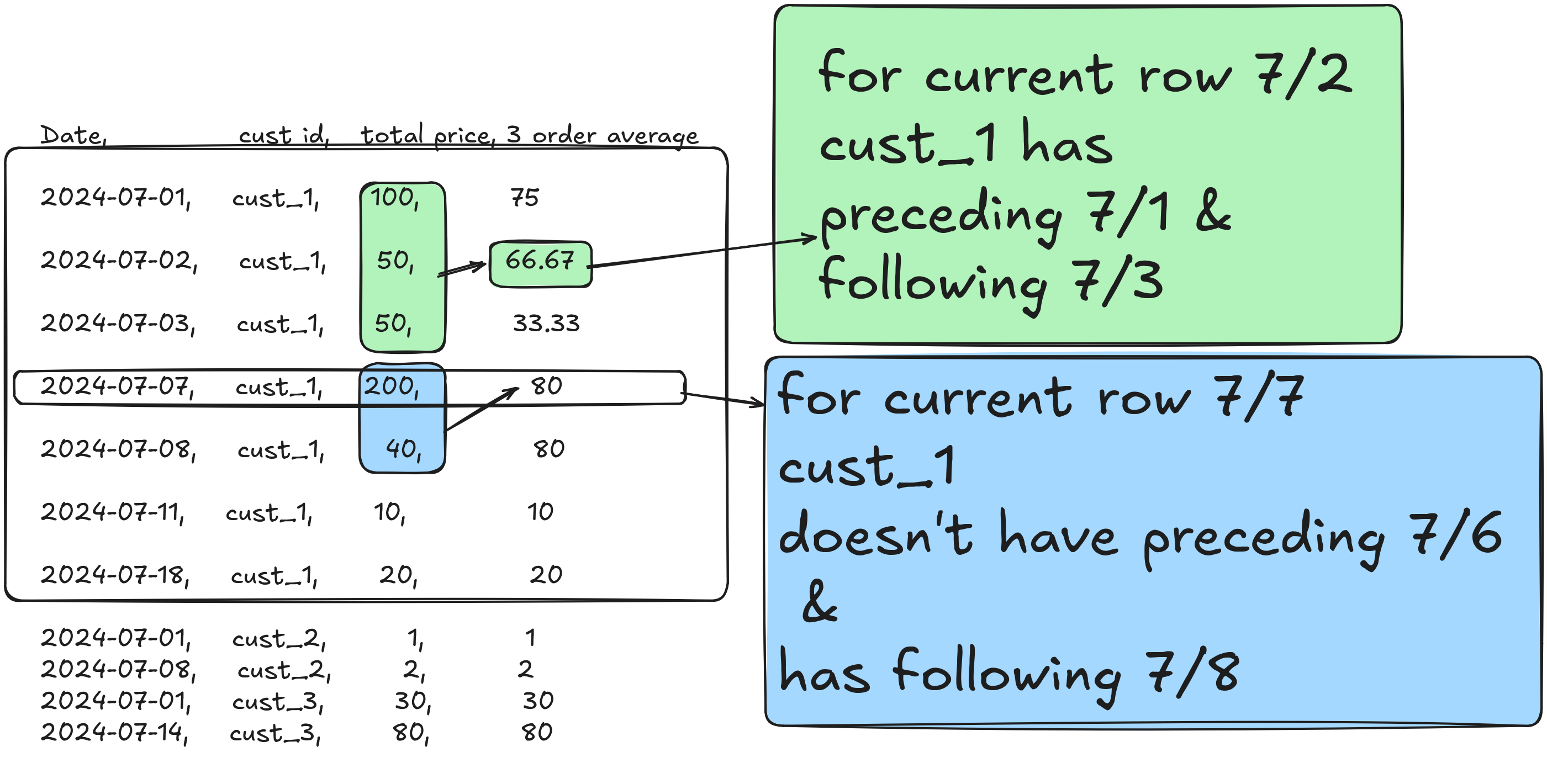
3.2.0.2 Use values of the columns to define the window frame using the RANGE clause

RANGE: Used to select a set of rows relative to the current row based on the value of the columns specified in the ORDER BY clause.
1. Range definition format: RANGE BETWEEN start_point AND end_point.
2. The start_point and end_point can be any of the following:
  1. CURRENT ROW: The current row.
  2. n PRECEDING: All rows with values within the specified range that are less than or equal to n units preceding the value of the current row.
  3. n FOLLOWING: All rows with values within the specified range that are greater than or equal to n units following the value of the current row.
  4. UNBOUNDED PRECEDING: All rows before the current row within the partition.
  5. UNBOUNDED FOLLOWING: All rows after the current row within the partition.
3. RANGE is handy when dealing with numeric or date/time ranges, allowing for calculations like running totals, moving averages, or cumulative distributions.

Let’s see how RANGE works with AVG(total price) OVER (PARTITION BY customer id ORDER BY date RANGE BETWEEN INTERVAL '1' DAY PRECEDING AND '1' DAY FOLLOWING) using the below visualization:

3.3 Ranking functions enable you to rank your rows based on an order by clause

If you are working on a problem to retrieve the top/bottom n rows (as defined by a specific value), then use the row functions.

Let’s look at an example of how to use a row function:

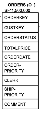
From the orders table get the top 3 spending customers per day. The orders table schema is shown below:

%%sql
SELECT
  *
FROM
  (
    SELECT
      o_orderdate,
      o_totalprice,
      o_custkey,
      RANK() -- RANKING FUNCTION 
      OVER (
        PARTITION BY
          o_orderdate -- PARTITION BY order date
        ORDER BY
          o_totalprice DESC -- ORDER rows withing partition by totalprice
      ) AS rnk
    FROM
      orders
  )
WHERE
  rnk <= 3
ORDER BY
  o_orderdate
LIMIT
  5;

Standard RANKING functions:

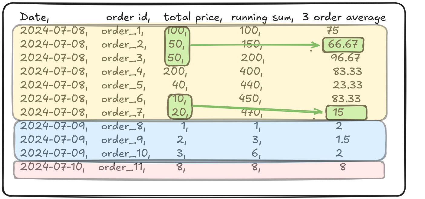
RANK: Ranks the rows starting from 1 to n within the window frame. Ranks the rows with the same value (defined by the “ORDER BY” clause) as the same and skips the ranking numbers that would have been present if the values were different.
DENSE_RANK: Ranks the rows starting from 1 to n within the window frame. Ranks the rows with the same value (defined by the “ORDER BY” clause) as the same and does not skip any ranking numbers.
ROW_NUMBER: Adds a row number that starts from 1 to n within the window frame and does not create any repeating values.

%%sql
-- Let's look at an example showing the difference between RANK, DENSE_RANK and ROW_NUMBER
SELECT 
    order_date,
    order_id,
    total_price,
    ROW_NUMBER() OVER (PARTITION BY order_date ORDER BY total_price) AS row_number,
    RANK() OVER (PARTITION BY order_date ORDER BY total_price) AS rank,
    DENSE_RANK() OVER (PARTITION BY order_date ORDER BY total_price) AS dense_rank
FROM (
    SELECT 
        '2024-07-08' AS order_date, 'order_1' AS order_id, 100 AS total_price UNION ALL
    SELECT 
        '2024-07-08', 'order_2', 200 UNION ALL
    SELECT 
        '2024-07-08', 'order_3', 150 UNION ALL
    SELECT 
        '2024-07-08', 'order_4', 90 UNION ALL
    SELECT 
        '2024-07-08', 'order_5', 100 UNION ALL
    SELECT 
        '2024-07-08', 'order_6', 90 UNION ALL
    SELECT 
        '2024-07-08', 'order_7', 100 UNION ALL
    SELECT 
        '2024-07-10', 'order_8', 100 UNION ALL
    SELECT 
        '2024-07-10', 'order_9', 100 UNION ALL
    SELECT 
        '2024-07-10', 'order_10', 100 UNION ALL
    SELECT 
        '2024-07-11', 'order_11', 100
) AS orders
ORDER BY order_date, row_number;

3.4 Aggregate functions enable you to compute running metrics

The standard aggregate functions are MIN, MAX, AVG, SUM, & COUNT. In addition to these, make sure to check your DB engine documentation, in our case, Spark Aggregate functions.

When you need a running sum/min/max/avg, it’s almost always a use case for aggregate functions with windows.

Let’s look at an example:

Write a query on the orders table that has the following output:
1. o_custkey
2. order_month: In YYYY-MM format, use strftime(o_orderdate, ‘%Y-%m’) AS order_month
3. total_price: Sum of o_totalprice for that month
4. three_mo_total_price_avg: The 3 month (previous, current & next) average of total_price for that customer

%%sql
SELECT
  order_month,
  o_custkey,
  total_price,
  ROUND(
    AVG(total_price) OVER ( -- FUNCTION: RUNNING AVERAGE
      PARTITION BY
        o_custkey -- PARTITIONED BY customer
      ORDER BY
        order_month ROWS BETWEEN 1 PRECEDING
        AND 1 FOLLOWING -- WINDOW FRAME DEFINED AS 1 ROW PRECEDING to 1 ROW FOLLOWING
    ),
    2
  ) AS three_mo_total_price_avg
FROM
  (
    SELECT
      date_format(o_orderdate, 'yyyy-MM') AS order_month,
      o_custkey,
      SUM(o_totalprice) AS total_price
    FROM
      orders
    GROUP BY
      1,
      2
  )
LIMIT
  5;

Now that we have seen how to define a window function and how to use ranking and aggregation functions, let’s take it a step further by practicing value functions.

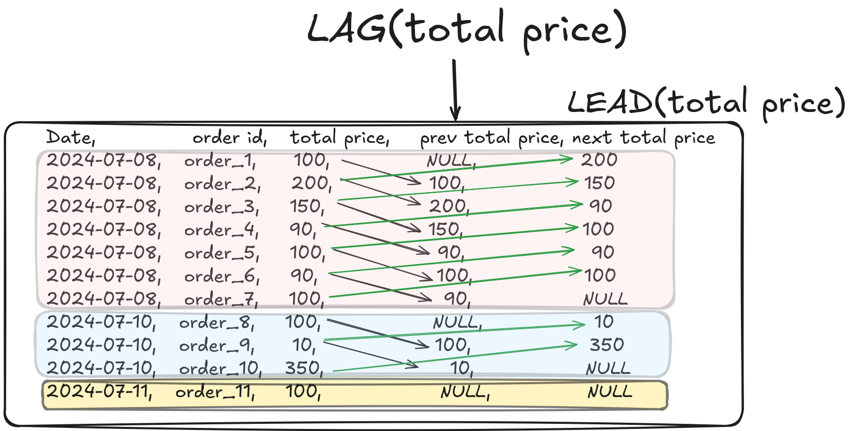
Remember that value functions are used to access the values of other rows while operating on the current row.

Let’s take a look at LEAD and LAG functions:

3.5 Value functions are used to access other rows’ values

Standard VALUE functions:

NTILE(n): Divides the rows in the window frame into n approximately equal groups, and assigns a number to each row indicating which group it belongs to.
FIRST_VALUE(): Returns the first value in the window frame.
LAST_VALUE(): Returns the last value in the window frame.
LAG(): Accesses data from a previous row within the window frame.
LEAD(): Accesses data from a subsequent row within the window frame.

3.6 Exercises

Write a query on the orders table that has the following output:
1. order_month,
2. o_custkey,
3. total_price,
4. three_mo_total_price_avg
5. consecutive_three_mo_total_price_avg: The consecutive 3 month average of total_price for that customer. Note that this should only include months that are chronologically next to each other.

Hint: Use CAST(strftime(o_orderdate, '%Y-%m-01') AS DATE) to cast order_month to date format.

Hint: Use the INTERVAL format shown above to construct the window function to compute consecutive_three_mo_total_price_avg column.

The orders table schema is shown below:

From the orders table get the 3 lowest spending customers per day

Hint: Figure out the PARTITION BY column first, then the ORDER BY column and finally the FUNCTION to use to compute running average.

Write a SQL query using the orders table that calculates the following columns:
1. o_orderdate: From orders table
2. o_custkey: From orders table
3. o_totalprice: From orders table
4. totalprice_diff: The customers current day’s o_totalprice - that same customers most recent previous purchase’s o_totalprice

Hint: Start by figuring out what the PARTITION BY column should be, then what the ORDER BY column should be, and then finally the function to use.

Hint: Use the LAG(column_name) ranking function to identify the prior day’s revenue.

3.7 Recommended reading

Window SQL Youtube workshop