1  Read data, Combine tables, & aggregate numbers to understand business performance

1.1 Setup

To run the code, you need to generate the data and load it into Spark tables. Use the script below to do this:

%%capture
%%bash
python ./generate_data.py
python ./run_ddl.py

%%sql --show
use prod.db

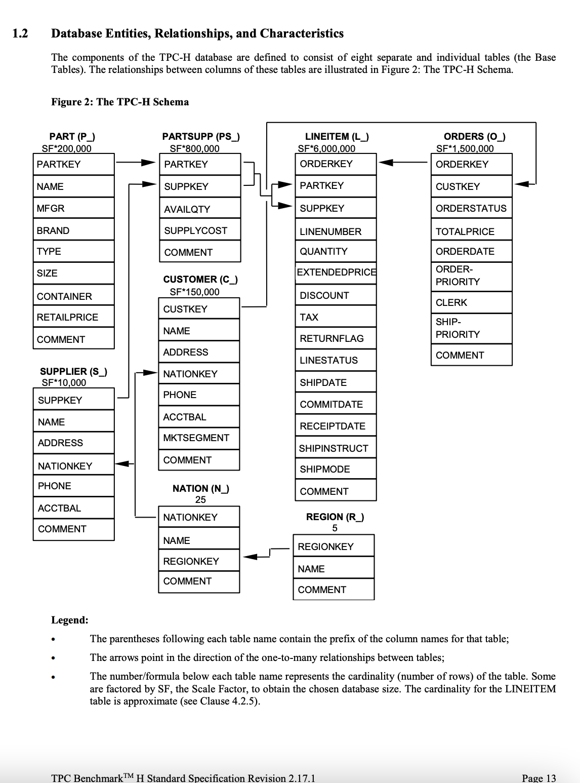
1.2 A Spark catalog can have multiple schemas, & schemas can have multiple tables

In Spark you can have multiple catalogs, each with multiple schemas and each schema with multiple tables.

The hierarchy in modern catalog systems is Catalog → Schema → Table .

%%sql 
show catalogs;

%%sql
show schemas IN demo;

-- Catalog -> schema

%%sql
show schemas IN prod;

-- schema -> namespace

%%sql
show tables IN prod.db -- namespace -> Table

%%sql --show
select * from prod.db.customer limit 2

Note how, when referencing the table name, we use the full path, i.e., schema.table_name. We can skip using the full path of the table if we define which schema to use for the entirety of this session, as shown below.

%%sql --show
use prod.db

%%sql
DESCRIBE lineitem

%%sql
DESCRIBE extended lineitem

1.3 Use SELECT…FROM, LIMIT, WHERE, & ORDER BY to read the required data

The most common use for querying is to read data from our tables. We can do this using a SELECT ... FROM statement, as shown below.

%%sql
-- use * to specify all columns
SELECT
  *
FROM
  orders
LIMIT
  4

%%sql
-- use column names to only read data from those columns
SELECT
  o_orderkey,
  o_totalprice
FROM
  orders
LIMIT
  4

However, running a SELECT ... FROM statement can cause issues when the data set is extensive. If you want to examine the data, use LIMIT n to instruct Trino to retrieve only the first n rows.

We can use the ‘WHERE’ clause to retrieve rows that match specific criteria. We can specify one or more filters within the’ WHERE’ clause. The WHERE clause with more than one filter can use combinations of AND and OR criteria to combine the filter criteria, as shown below.

%%sql
-- all customer rows that have c_nationkey = 20
SELECT
  *
FROM
  customer
WHERE
  c_nationkey = 20
LIMIT
  10;

%%sql
-- all customer rows that have c_nationkey = 20 and c_acctbal > 1000
SELECT
  *
FROM
  customer
WHERE
  c_nationkey = 20
  AND c_acctbal > 1000
LIMIT
  10;

%%sql
-- all customer rows that have c_nationkey = 20 or c_acctbal > 1000
SELECT
  *
FROM
  customer
WHERE
  c_nationkey = 20
  OR c_acctbal > 1000
LIMIT
  10;

%%sql
-- all customer rows that have (c_nationkey = 20 and c_acctbal > 1000) or rows that have c_nationkey = 11
SELECT
  *
FROM
  customer
WHERE
  (
    c_nationkey = 20
    AND c_acctbal > 1000
  )
  OR c_nationkey = 11
LIMIT
  10;

We can combine multiple filter clauses, as seen above. We have seen examples of equals (=) and greater than (>) conditional operators. There are 6 conditional operators, they are

1. < Less than
2. > Greater than
3. <= Less than or equal to
4. >= Greater than or equal to
5. = Equal
6. <> and != both represent Not equal (some DBs only support one of these)

Additionally, for string types, we can make pattern matching with like condition. In a like condition, a _ means any single character, and % means zero or more characters, for example.

%%sql
-- all customer rows where the name has a 381 in it
SELECT
  *
FROM
  customer
WHERE
  c_name LIKE '%381%';

%%sql
-- all customer rows where the name ends with a 381
SELECT
  *
FROM
  customer
WHERE
  c_name LIKE '%381';

%%sql
-- all customer rows where the name starts with a 381
SELECT
  *
FROM
  customer
WHERE
  c_name LIKE '381%';

%%sql
-- all customer rows where the name has a combination of any character and 9 and 1
SELECT
  *
FROM
  customer
WHERE
  c_name LIKE '%_91%';

We can also filter for more than one value using IN and NOT IN.

%%sql
-- all customer rows which have nationkey = 10 or nationkey = 20
SELECT
  *
FROM
  customer
WHERE
  c_nationkey IN (10, 20);

%%sql
-- all customer rows which have do not have nationkey as 10 or 20
SELECT
  *
FROM
  customer
WHERE
  c_nationkey NOT IN (10, 20);

We can get the number of rows in a table using count(*) as shown below.

%%sql
SELECT
  COUNT(*)
FROM
  customer;

-- 1500

%%sql
SELECT
  COUNT(*)
FROM
  lineitem;

-- 60175

If we want to get the rows sorted by values in a specific column, we use ORDER BY, for example.

%%sql
-- Will show the first ten customer records with the lowest custkey
-- rows are ordered in ASC order by default
SELECT
  *
FROM
  orders
ORDER BY
  o_custkey
LIMIT
  10;

%%sql
-- Will show the first ten customer's records with the highest custkey
SELECT
  *
FROM
  orders
ORDER BY
  o_custkey DESC
LIMIT
  10;

1.4 Combine data from multiple tables using JOINs

We can combine data from multiple tables using joins. When we write a join query, we have a format as shown below.

SELECT
    a.*
FROM
    table_a a -- LEFT table a
    JOIN table_b b -- RIGHT table b
    ON a.id = b.id

The table specified first (table_a) is the left table, whereas the table specified second is the right table. When we have multiple tables joined, we consider the joined dataset from the first two tables as the left table and the third table as the right table (The DB optimizes our join for performance).

SELECT
    a.*
FROM
    table_a a -- LEFT table a
    JOIN table_b b -- RIGHT table b
    ON a.id = b.id
    JOIN table_c c -- LEFT table is the joined data from table_a & table_b, right table is table_c
    ON a.c_id = c.id

There are five main types of joins:

Join Types

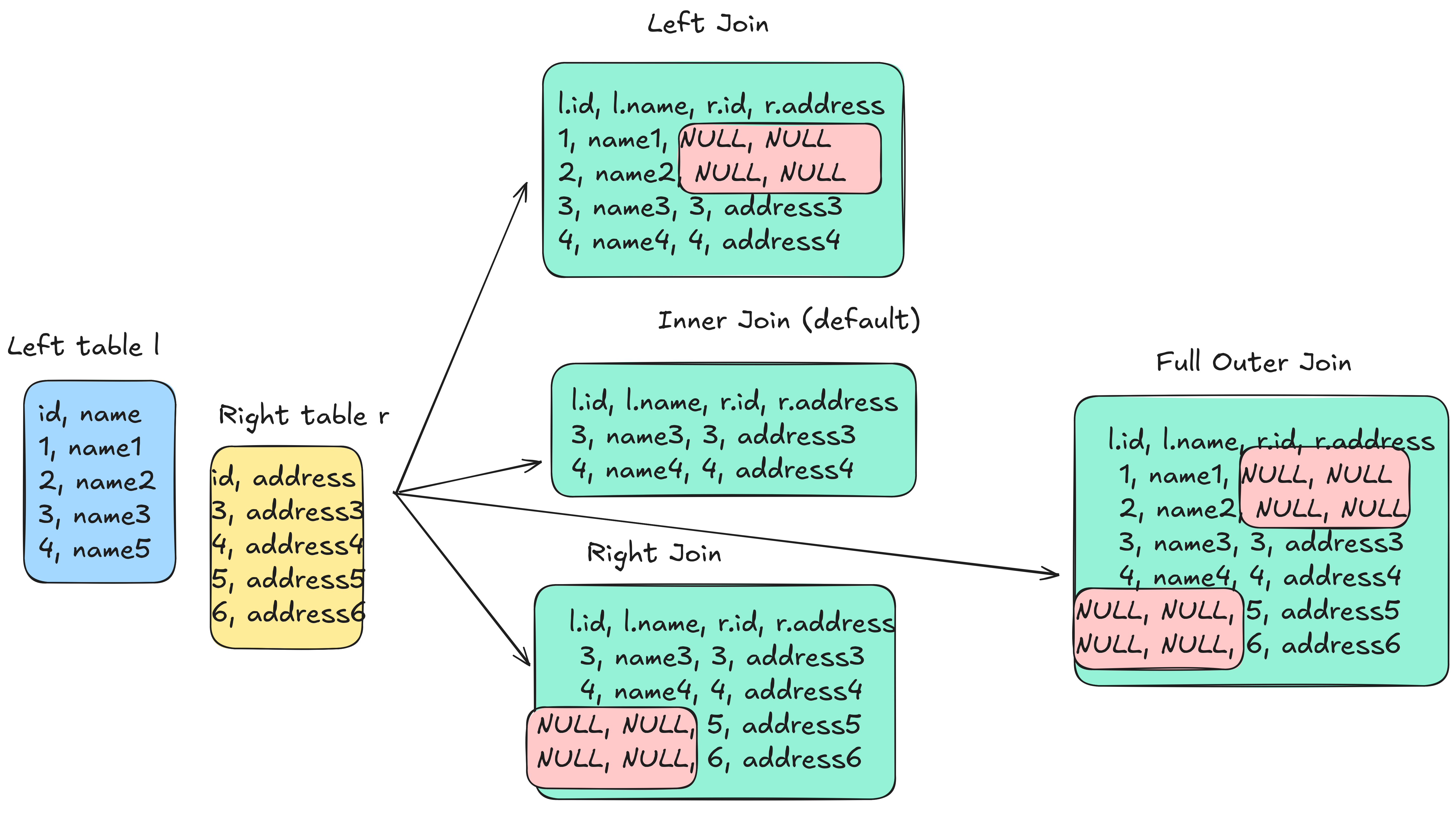
1.4.1 1. Inner join (default): Get rows with the same join keys from both tables

%%sql
SELECT
  o.o_orderkey,
  l.l_orderkey
FROM
  orders o
  JOIN lineitem l ON o.o_orderkey = l.l_orderkey
  AND o.o_orderdate BETWEEN l.l_shipdate - INTERVAL '5' DAY AND l.l_shipdate  + INTERVAL '5' DAY
LIMIT
  10;

%%sql
SELECT
  COUNT(o.o_orderkey) AS order_rows_count,
  COUNT(l.l_orderkey) AS lineitem_rows_count
FROM
  orders o
  JOIN lineitem l ON o.o_orderkey = l.l_orderkey
  AND o.o_orderdate BETWEEN l.l_shipdate - INTERVAL '5' DAY AND l.l_shipdate  + INTERVAL '5' DAY;
-- 2477, 2477

Note: JOIN defaults to INNER JOIN`.

The output will contain rows from orders and lineitem that match at least one row from the other table with the specified join condition (same orderkey and orderdate within a 5-day window of the ship date).

We can also see that 2,477 rows from the orders and lineitem tables matched.

1.4.2 2. Left outer join (aka left join): Get all rows from the left table and only matching rows from the right table.

%%sql

SELECT
  o.o_orderkey,
  l.l_orderkey
FROM
  orders o
  LEFT JOIN lineitem l ON o.o_orderkey = l.l_orderkey
  AND o.o_orderdate BETWEEN l.l_shipdate - INTERVAL '5' DAY AND l.l_shipdate  + INTERVAL '5' DAY
LIMIT
  10;

%%sql
SELECT
  COUNT(o.o_orderkey) AS order_rows_count,
  COUNT(l.l_orderkey) AS lineitem_rows_count
FROM
  orders o
  LEFT JOIN lineitem l ON o.o_orderkey = l.l_orderkey
  AND o.o_orderdate BETWEEN l.l_shipdate - INTERVAL '5' DAY AND l.l_shipdate  + INTERVAL '5' DAY;
-- 15197, 2477

The output will include all rows from orders and the rows from lineitem that were able to find at least one matching row from the orders table with the specified join condition (same orderkey and orderdate within a 5-day window of the ship date).

We can also see that the number of rows from the orders table is 15,197 & from the lineitem table is 2,477. The number of rows in orders is 15,000, but the join condition produces 15,197 since some orders match with multiple line items.

1.4.3 3. Right outer join (aka right join): Get matching rows from the left and all rows from the right table.

%%sql
SELECT
  o.o_orderkey,
  l.l_orderkey
FROM
  orders o
  RIGHT JOIN lineitem l ON o.o_orderkey = l.l_orderkey
  AND o.o_orderdate BETWEEN l.l_shipdate - INTERVAL '5' DAY AND l.l_shipdate  + INTERVAL '5' DAY
LIMIT
  10;

%%sql
SELECT
  COUNT(o.o_orderkey) AS order_rows_count,
  COUNT(l.l_orderkey) AS lineitem_rows_count
FROM
  orders o
  RIGHT JOIN lineitem l ON o.o_orderkey = l.l_orderkey
  AND o.o_orderdate BETWEEN l.l_shipdate - INTERVAL '5' DAY AND l.l_shipdate  + INTERVAL '5' DAY;
-- 2477, 60175

The output will include the rows from orders that match at least one row from the lineitem table with the specified join condition (same orderkey and orderdate within a 5-day window of the ship date) and all rows from the lineitem table.

We can also see that the number of rows from the orders table is 15,197 & from the lineitem table is 2,477.

1.4.4 4. Full outer join: Get matched and unmatched rows from both tables.

%%sql
SELECT
  o.o_orderkey,
  l.l_orderkey
FROM
  orders o
  FULL OUTER JOIN lineitem l ON o.o_orderkey = l.l_orderkey
  AND o.o_orderdate BETWEEN l.l_shipdate - INTERVAL '5' DAY AND l.l_shipdate  + INTERVAL '5' DAY
LIMIT
  10

%%sql
SELECT
  COUNT(o.o_orderkey) AS order_rows_count,
  COUNT(l.l_orderkey) AS lineitem_rows_count
FROM
  orders o
  FULL OUTER JOIN lineitem l ON o.o_orderkey = l.l_orderkey
  AND o.o_orderdate BETWEEN l.l_shipdate - INTERVAL '5' DAY AND l.l_shipdate  + INTERVAL '5' DAY;
-- 15197, 60175

The output will include all rows from orders that match at least one row from the lineitem table with the specified join condition (same orderkey and orderdate within a 5-day window of the ship date) and all rows from the lineitem table.

We can also see that the number of rows from the orders table is 15,197 & from the lineitem table is 2,477.

1.4.5 5. Cross join: Join every row in the left table with every row in the right table

%%sql
SELECT
  n.n_name AS nation_c_name,
  r.r_name AS region_c_name
FROM
  nation n
  CROSS JOIN region r;

The output will have every row of the nation joined with every row of the region. There are 25 nations and five regions, leading to 125 rows in our result from the cross-join.

There are cases where we need to join a table with itself, known as a SELF-join. Let’s consider an example.

1. For every customer order, get the order placed earlier in the same week (Sunday - Saturday, not the previous seven days). Only show customer orders that have at least one such order.

%%sql    
SELECT
    o1.o_custkey as o1_custkey,
    o1.o_totalprice as o1_totalprice,
    o1.o_orderdate as o1_orderdate,
    o2.o_totalprice as o2_totalprice,
    o2.o_orderdate as o2_orderdate
FROM
    orders o1
    JOIN orders o2 ON o1.o_custkey = o2.o_custkey
    AND year(o1.o_orderdate) = year(o2.o_orderdate)
    AND weekofyear(o1.o_orderdate) = weekofyear(o2.o_orderdate)
WHERE
    o1.o_orderkey != o2.o_orderkey
LIMIT
    10;

1.5 Combine data from multiple rows into one using GROUP BY

Most analytical queries require calculating metrics that involve combining data from multiple rows. GROUP BY allows us to perform aggregate calculations on data from a set of rows recognized by values of specified column(s).

Let’s look at an example question:

1. Create a report that shows the number of orders per orderpriority segment.

%%sql
SELECT
  o_orderpriority,
  COUNT(*) AS num_orders
FROM
  orders
GROUP BY
  o_orderpriority;

In the above query, we group the data by orderpriority, and the calculation count(*) will be applied to the rows having a specific orderpriority value.

The calculations allowed are typically SUM/MIN/MAX/AVG/COUNT. However, some databases have more complex aggregate functions; check your DB documentation.

1.5.1 Use HAVING to filter based on the aggregates created by GROUP BY

If you want to filter based on the values of an aggregate function from a group by, use the having clause. Note that the having clause should come after the group by clause.

%%sql
SELECT
  o_orderpriority,
  COUNT(*) AS num_orders
FROM
  orders
GROUP BY
  o_orderpriority
HAVING
    COUNT(*) > 3;

1.6 Replicate IF.ELSE logic with CASE statements

We can do conditional logic in the SELECT ... FROM part of our query, as shown below.

%%sql
SELECT
    o_orderkey,
    o_totalprice,
    CASE
        WHEN o_totalprice > 100000 THEN 'high'
        WHEN o_totalprice BETWEEN 25000
        AND 100000 THEN 'medium'
        ELSE 'low'
    END AS order_price_bucket
FROM
    orders;

We can see how we display different values depending on the totalprice column. We can also use multiple criteria as our conditional criteria (e.g., totalprice > 100000 AND orderpriority = ‘2-HIGH’).

1.7 Stack tables on top of each other with UNION and UNION ALL, subtract tables with EXCEPT

When we want to combine data from tables by stacking them on top of each other, we use the UNION or UNION ALL operator. UNION removes duplicate rows, and UNION ALL does not remove duplicate rows. Let’s look at an example.

%%sql
SELECT c_custkey, c_name FROM customer WHERE c_name LIKE '%_91%' -- 25 rows

%%sql
-- UNION will remove duplicate rows; the below query will produce 25 rows
SELECT c_custkey, c_name FROM customer WHERE c_name LIKE'%_91%'
UNION
SELECT c_custkey, c_name FROM customer WHERE c_name LIKE '%_91%'
UNION
SELECT c_custkey, c_name FROM customer WHERE c_name LIKE '%_91'
LIMIT 10;

%%sql
-- UNION ALL will not remove duplicate rows; the below query will produce 75 rows
SELECT c_custkey, c_name FROM customer WHERE c_name LIKE '%_91%'
UNION ALL
SELECT c_custkey, c_name FROM customer WHERE c_name LIKE '%_91%'
UNION ALL
SELECT c_custkey, c_name FROM customer WHERE c_name LIKE '%_91%'
LIMIT 10;

When we want to retrieve all rows from the first dataset that are not present in the second dataset, we can use EXCEPT.

%%sql
-- EXCEPT will get the rows in the first query result that is not in the second query result, 0 rows
SELECT c_custkey, c_name FROM customer WHERE c_name LIKE '%_91%'
EXCEPT
SELECT c_custkey, c_name FROM customer WHERE c_name LIKE '%_91%'
LIMIT 10;

%%sql
-- The below query will result in 23 rows; the first query has 25 rows, and the second has two rows
SELECT c_custkey, c_name FROM customer WHERE c_name LIKE'%_91%'
EXCEPT
SELECT c_custkey, c_name FROM customer WHERE c_name LIKE '%191%'
LIMIT 10;

1.8 Sub-query: Use a query instead of a table

When we want to use the result of a query as a table in another query, we use subqueries. Let’s consider an example:

1. Create a report that shows the nation, how many items it supplied (by suppliers in that nation), and how many items it purchased (by customers in that nation).

%%sql
SELECT
  n.n_name AS nation_c_name,
  s.quantity AS supplied_items_quantity,
  c.quantity AS purchased_items_quantity
FROM
  nation n
  LEFT JOIN (
    SELECT
      n.n_nationkey,
      SUM(l.l_quantity) AS quantity
    FROM
      lineitem l
      JOIN supplier s ON l.l_suppkey = s.s_suppkey
      JOIN nation n ON s.s_nationkey = n.n_nationkey
    GROUP BY
      n.n_nationkey
  ) s ON n.n_nationkey = s.n_nationkey
  LEFT JOIN (
    SELECT
      n.n_nationkey,
      SUM(l.l_quantity) AS quantity
    FROM
      lineitem l
      JOIN orders o ON l.l_orderkey = o.o_orderkey
      JOIN customer c ON o.o_custkey = c.c_custkey
      JOIN nation n ON c.c_nationkey = n.n_nationkey
    GROUP BY
      n.n_nationkey
  ) c ON n.n_nationkey = c.n_nationkey;

In the above query, we can see that there are two sub-queries, one to calculate the quantity supplied by a nation and the other to calculate the quantity purchased by the customers of a nation.

1.9 Change data types (CAST) and handle NULLS (COALESCE)

Every column in a table has a specific data type. The data types fall under one of the following categories.

1. Numerical: Data types used to store numbers.
   1. Integer: Positive and negative numbers. Different types of Integer, such as tinyint, int, and bigint, allow storage of different ranges of values. Integers cannot have decimal digits.
   2. Floating: These can have decimal digits but store an approximate value.
   3. Decimal: These can have decimal digits and store the exact value. The decimal type allows you to specify the scale and precision. Where scale denotes the count of numbers allowed as a whole & precision denotes the count of numbers allowed after the decimal point. E.g., DECIMAL(8,3) allows eight numbers in total, with three allowed after the decimal point.
2. Boolean: Data types used to store True or False values.
3. String: Data types used to store alphanumeric characters.
   1. Varchar(n): Data type allows storage of a variable character string, with a permitted max length n.
   2. Char(n): Data type allows storage of a fixed character string. A column of char(n) type adds (length(string) - n) empty spaces to a string that does not have n characters.
4. Date & time: Data types used to store dates, time, & timestamps(date + time).
5. Objects (STRUCT, ARRAY, MAP, JSON): Data types used to store JSON and ARRAY data.

Some databases have data types that are unique to them as well. We should check the database documents to understand the data types offered.

It is best practice to use the appropriate data type for your columns. We can convert data types using the CAST function, as shown below.

A NULL will be used for that field when a value is not present. In cases where we want to use the first non-NULL value from a list of columns, we use COALESCE as shown below.

Let’s consider the following example. We can see how when l.orderkey is NULL, the DB uses 999999 as the output.

%%sql
SELECT
    o.o_orderkey,
    o.o_orderdate,
    COALESCE(l.l_orderkey, 9999999) AS lineitem_orderkey,
    l.l_shipdate
FROM
    orders o
    LEFT JOIN lineitem l ON o.o_orderkey = l.l_orderkey
    AND o.o_orderdate BETWEEN l.l_shipdate - INTERVAL '5' DAY
    AND l.l_shipdate + INTERVAL '5' DAY
LIMIT
    10;

1.10 Use these standard inbuilt DB functions for String, Time, and Numeric data manipulation

When processing data, more often than not, we will need to change values in columns; shown below are a few standard functions to be aware of:

1. String functions
   1. LENGTH is used to calculate the length of a string. E.g., SELECT LENGTH('hi'); will output 2.
   2. CONCAT combines multiple string columns into one. E.g., SELECT CONCAT(clerk, '-', orderpriority) FROM ORDERS LIMIT 5; will concatenate clerk and orderpriority columns with a dash in between them.
   3. SPLIT is used to split a value into an array based on a given delimiter. E.g., SELECT SPLIT(clerk, '#') FROM ORDERS LIMIT 5; will output a column with arrays formed by splitting clerk values on #.
   4. SUBSTRING is used to get a sub-string from a value, given the start and length. E.g., SELECT clerk, SUBSTRING(clerk, 1, 5) FROM orders LIMIT 5; will get the first five characters of the clerk column. Note that indexing starts from 1 in Spark SQL.
   5. TRIM is used to remove empty spaces to the left and right of the value. E.g., SELECT TRIM(' hi '); will output hi without any spaces around it. LTRIM and RTRIM are similar but only remove spaces before and after the string, respectively.
2. Date and Time functions

   1. Adding and subtracting dates: Is used to add and subtract periods; the format heavily depends on the DB. E.g., In Spark SQL, the query

        SELECT
        DATEDIFF(DATE '2023-11-05', DATE '2022-10-01') AS diff_in_days,
        MONTHS_BETWEEN(DATE '2023-11-05', DATE '2022-10-01') AS diff_in_months,
        YEAR(DATE '2023-11-05') - YEAR(DATE '2022-10-01') AS diff_in_years;

      It will show the difference between the two dates in the specified period. We can also add/subtract an arbitrary period from a date/time column. E.g., SELECT DATE_ADD(DATE '2022-11-05', 10); will show the output 2022-11-15.

   2. string <=> date/time conversions: When we want to change the data type of a string to date/time, we can use the DATE 'YYYY-MM-DD' or TIMESTAMP 'YYYY-MM-DD HH:mm:SS' functions. But when the data is in a different date/time format such as MM/DD/YYYY, we will need to specify the input structure; we do this using TO_DATE or TO_TIMESTAMP. E.g. SELECT TO_DATE('11-05-2023', 'MM-dd-yyyy');. We can convert a timestamp/date into a string with the required format using DATE_FORMAT. E.g., SELECT DATE_FORMAT(orderdate, 'yyyy-MM-01') AS first_month_date FROM orders LIMIT 5; will map every orderdate to the first of their month.

   3. Time frame functions (YEAR/MONTH/DAY): When we want to extract specific periods from a date/time column, we can use these functions. E.g., SELECT YEAR(DATE '2023-11-05'); will return 2023. Similarly, we have MONTH, DAY, HOUR, MINUTE, etc.

3. Numeric
   1. ROUND is used to specify the number of digits allowed after the decimal point. E.g. SELECT ROUND(100.102345, 2);

1.11 Save queries as views for more straightforward reads

When we have large/complex queries that we need to run often, we can save them as views. Views are database objects that operate similarly to tables. The OLAP DB executes the underlying query when we query a view.

Use views to hide query complexities and limit column access (by exposing only specific table columns) for end-users.

For example, we can create a view for the nation-level report from the above section, as shown below.

%%sql
DROP VIEW IF EXISTS nation_supplied_purchased_quantity

%%sql
CREATE VIEW nation_supplied_purchased_quantity AS
SELECT
    n.n_name AS nation_name,
    s.quantity AS supplied_items_quantity,
    c.quantity AS purchased_items_quantity
FROM
    nation n
    LEFT JOIN (
        SELECT
            n_nationkey as nationkey,
            sum(l_quantity) AS quantity
        FROM
            lineitem l
            JOIN supplier s ON l.l_suppkey = s.s_suppkey
            JOIN nation n ON s.s_nationkey = n.n_nationkey
        GROUP BY
            n.n_nationkey
    ) s ON n.n_nationkey = s.nationkey
    LEFT JOIN (
        SELECT
            n_nationkey as nationkey,
            sum(l_quantity) AS quantity
        FROM
            lineitem l
            JOIN orders o ON l.l_orderkey = o.o_orderkey
            JOIN customer c ON o.o_custkey = c.c_custkey
            JOIN nation n ON c.c_nationkey = n.n_nationkey
        GROUP BY
            n.n_nationkey
    ) c ON n.n_nationkey = c.nationkey;

%%sql
SELECT
    *
FROM
    nation_supplied_purchased_quantity;

Now the view nation_supplied_purchased_quantity will run the underlying query when used.

1.12 Exercises

1. Write a query that shows the number of items returned for each region name
2. List the top 10 most selling parts (part name)
3. Sellers (name) who have sold at least one of the top 10 selling parts
4. Number of items returned for each order price bucket. The definition of order price bucket is shown below.

CASE
    WHEN o_totalprice > 100000 THEN 'high'
    WHEN o_totalprice BETWEEN 25000 AND 100000 THEN 'medium'
    ELSE 'low'
END AS order_price_bucket

5. Average time (in days) between receiptdate and shipdate for each nation (name)

Here is the data model:

1.13 Recommended reading

1. Improving SQL Skills
2. SQL techniques
3. Advanced SQL skills