%%sql
use prod_db8 Data warehouse modeling (Kimball) is based off of 2 types of tables: Fact and dimensions
Data warehousing is more than just moving data to an OLAP database; the key part of data warehousing is data modeling.
Data modelling ensures that the data is suited for our specific use case(data analytics is our use case)
The data from source systems (your company’s backend, API data pulls, etc) is usually normalized & modeled for effective CRUD of a small number of rows at a time.
However, in a data warehouse, we usually want to aggregate a large number of rows based on a set of columns. For this use case, Kimball’s Dimensional model has been the most standard practice.
In this chapter, we will cover the basics of Kimball design with an eye towards modern infrastructure and expand on them.
8.1 Facts represent events that occured & dimension the entities to which events occur.
A data warehouse is a database that stores your company’s historical data. The main types of tables you need to create to power analytics are:
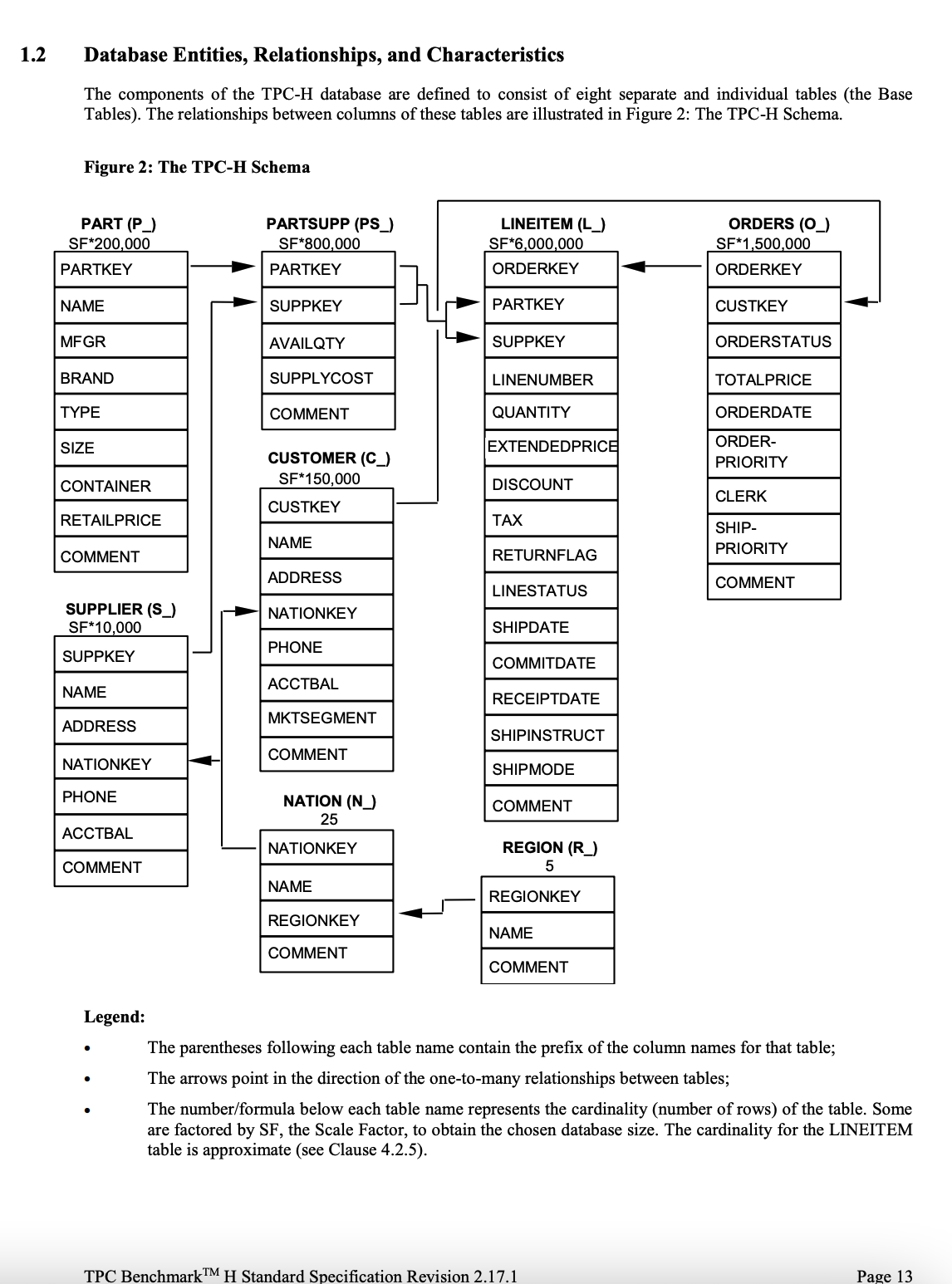
Dimension: Each row in a dimension table represents a business entity that is important to the business. For example, we have acustomerdimension table, where each row represents an individual customer. Other examples of dimension tables aresupplier&parttables.Facts: Each row in a fact table represents a business process that occurred. E.g., in our data warehouse, each row in theordersfact table will represent an individual order, and each row in thelineitemfact table will represent an item sold as part of an order. Each fact row will have a unique identifier; in our case, it’sorderkeyfor orders and a combination oforderkey & linenumberfor lineitem.
A table’s grain (aka granularity, level) refers to what a row of that table represents. For example, in our checkout process, we can have two fact tables: one for the order and another for the individual items in the order.
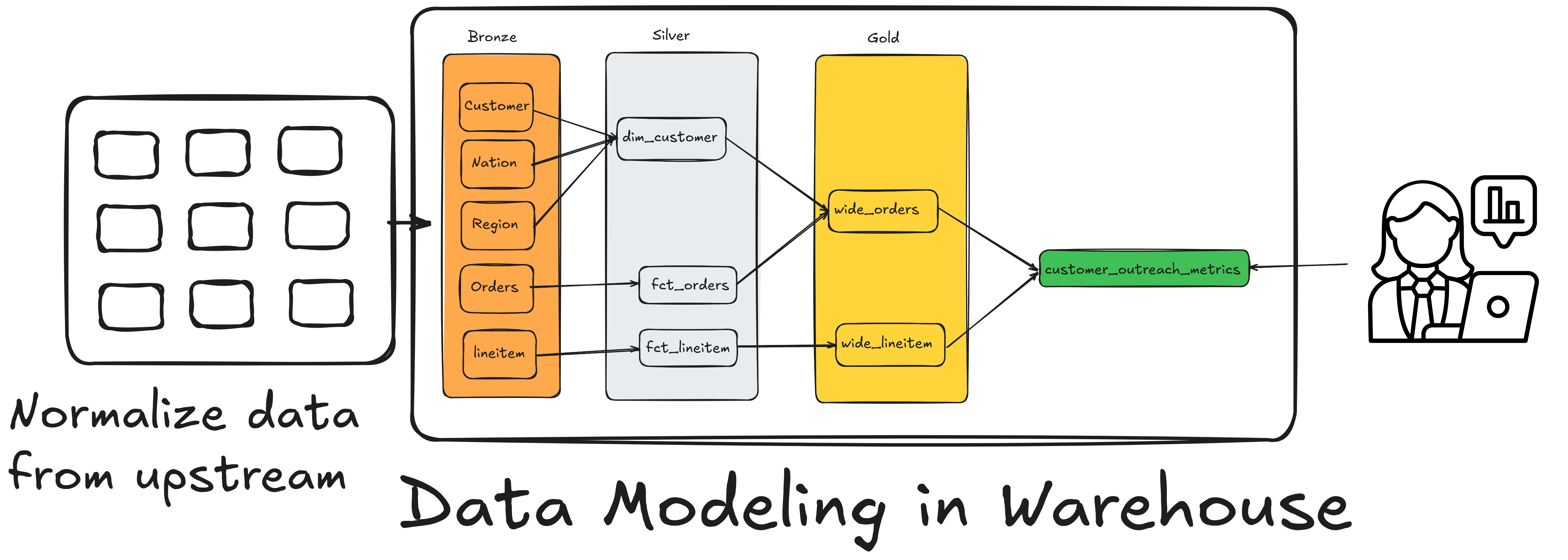
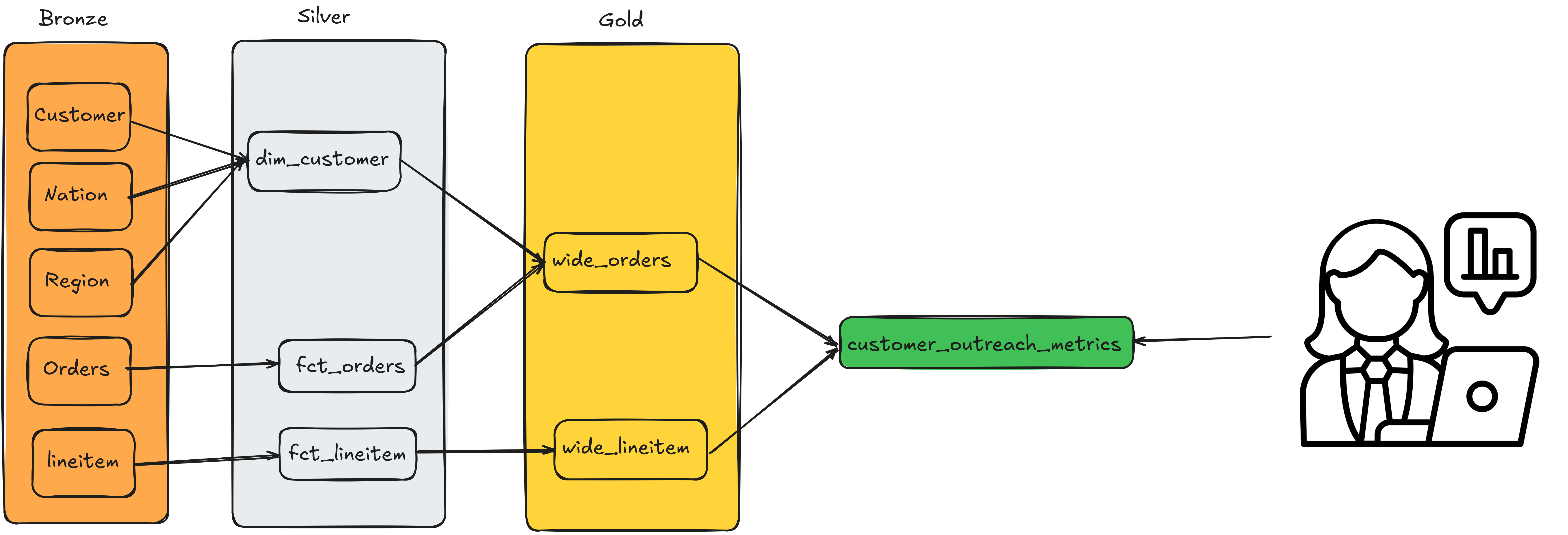
The items table will have one row for each item purchased, whereas the order table will have one row for each order placed. Our TPCH data is modelled into facts and dimensions as shown below:
%%sql
-- calculating the totalprice of an order (with orderkey = 1) from it's individual items
SELECT
    l_orderkey,
    round( sum(l_extendedprice * (1 - l_discount) * (1 + l_tax)),
        2
    ) AS totalprice
FROM
    lineitem
WHERE
    l_orderkey = 1
GROUP BY
l_orderkey;%%sql
-- The totalprice of an order (with orderkey = 1)
SELECT
o_orderkey,
o_totalprice
FROM
orders
WHERE
o_orderkey = 1;Note: If you notice the slight difference in the decimal digits, it’s due to using a double datatype, which is an inexact data type.
We can see how the lineitem table can be “rolled up” to get the data in the orders table. However, having just the orders table is insufficient, as the lineitem table provides us with individual item details, including discount and quantity information.
8.2 Popular dimension types: Full Snapshot & SCD2
Kimball defines Seven types of dimensional models; however, two of them are the most widely used.
Full snapshotIn this type of dimension, the entire dimension table is overwritten (or inserted with a specific load date) each run. Typically, each run creates a new copy while retaining the older copy for a specific period (e.g., 6 months). With the decreasing cost of storage, this is an acceptable tradeoff, especially since it is easy to implement and enables the users to go back in time.Slowly Changing Dimension Type 2, SCD2In this type of dimension, every change to the dimension’s entity (e.g, customer attribute change in a customer dimension) will result in a new row.
And every row will contain:
- valid_from: A timestamp column indicates the time from when this version of the customer attributes was valid.
- valid_to: A timestamp column indicates the time up to which this version of the customer attributes was valid.
- is_current: A boolean flag indicating if this row is the current state of the customer.
Consider this example where a supplier’s state changes from CA to IL (ref: Wiki)
| Supplier_Key | Supplier_Code | Supplier_Name | Supplier_State | Start_Date | End_Date | is_current |
|---|---|---|---|---|---|---|
| 123 | ABC | Acme Supply Co | CA | 2000-01-01T00:00:00 | 2004-12-22T00:00:00 | 0 |
| 123 | ABC | Acme Supply Co | IL | 2004-12-22T00:00:00 | NULL | 1 |
According to Kimball’s method, you are supposed to create a surrogate key (think of an ID that is continually increasing) for each row in the dimension and enrich the fact table with this dimension surrogate key to enable efficient joins.
However, in most modern data systems, the fact data flows in without too much delay and has the dimension’s unique key from upstream data. While the dimension tables may take a while to create.
With advances in data processing and partitioning formats, most companies skip the surrogate key modeling methodology and instead join based on the key from the upstream dataset and the time. See this how-to article for an example.
8.3 One Big Table (OBT) is a fact table left-joined with all its dimensions
As the number of facts and dimensions increases, you will notice that most queries used by end users to retrieve data utilize the same tables and joins.
In this scenario, the expensive reprocessing of data can be avoided by creating an OBT. In an OBT, you left-join all the dimensions into a fact table. This OBT can then be used to aggregate data to different grains as needed for end-user reporting.
Note that the OBT should have the exact grain as the lowest grain of the fact table that it is based on. In our bike-part seller warehouse, we can create an OBT for orders by joining all the tables to the lineitem table.
select
    f.*,
    d.other_attributes
from fct_orders as f
left join dim_customer as d on f.customer_key = d.customer_key
From the above image, we can see that the OBT tables are wide_orders and wide_lineitem.
8.4 Summary or pre-aggregated tables are stakeholder-team-specific tables built for reporting
Stakeholders often require data aggregated at various grains and similar metrics. Creating pre-aggregated or summary tables enables the generation of these reports for stakeholders, allowing them to select from the table without needing to recompute metrics.
The summary table has two key benefits.
- Consistent metric definition, as the data engineering will keep the metric definition in the code base, vs each stakeholder using a slightly different version and ending up with different numbers
- Avoid unnecessary recomputation, as multiple stakeholders can now use the same table
However, the downside is that the data may not be as fresh as what a stakeholder would obtain if they were to write a query.
Here is a simple example, assuming wide_lineitem is an OBT.
select
    order_key,
    COUNT(line_number) as num_lineitems
from wide_lineitem
group by order_key
From the above image, we can see that the summary table is customer_outreach_metrics.
8.5 Exercises
- What are the fact tables in our TPCH data model?
- What are the dimension tables in our TPCH data model?
- What source tables in the TPCH data model would you consider to create a customer dimension table?